In this chapter we will discuss the basic principles of fitting a model to data using the least squares method. We will use the CurveFit.jl package to perform the fitting.

Least squares fitting

You have some experimental data composed of $n$ pairs of data points $(x_i, y_i)$ where $i = 1, \dots, n$ and $y_i$ is the value that you observe at $x_i$. You want to gain some physical insight into the data by seeing how well a model explains it and adjusting the model parameters until the model function “fits” the data as best it can. For example, if you measure the absorbance for several samples of a liquid at various concentrations you expect there to be a linear relationship between the absorbance and the concentration (the famous Beer-Lambert Law). The difference between the measured absorbance and the linear model is the error. The slope and intercept of the line are the parameters to vary to find a line that best matches the data.

For whatever system you are studying, the parameters that produce a model that best fits the data hopefully say something useful about the physical system that you have measured. Aside from choosing a physically suitable model, we have to somehow quantify how well the model “fits” the data. The model function takes the form $f(p, x)$, where $p$ is a vector of parameters that you want to uncover via the fitting process. This vector of “best fit” parameters is what we are trying to find. How well the model fits the data is measured by the difference between the observed values $y_i$ and the model values $f(p, x_i)$ for a given $p$. The set of differences is called the residuals, and are defined by

$$r_i = y_i - f(p, x_i)$$

The least squares method then squares the residuals and sums them up. Minimizing this sum of the squared residuals will return the optimal parameters values $p$. The sum of the squared residuals is given by

$$S = \sum_{i=1}^n r_i^2 = \sum_{i=1}^n \left(y_i - f(p, x_i) \right)^2$$

This function is also known as the cost or loss function. Sometimes it is also referred to as the error function.

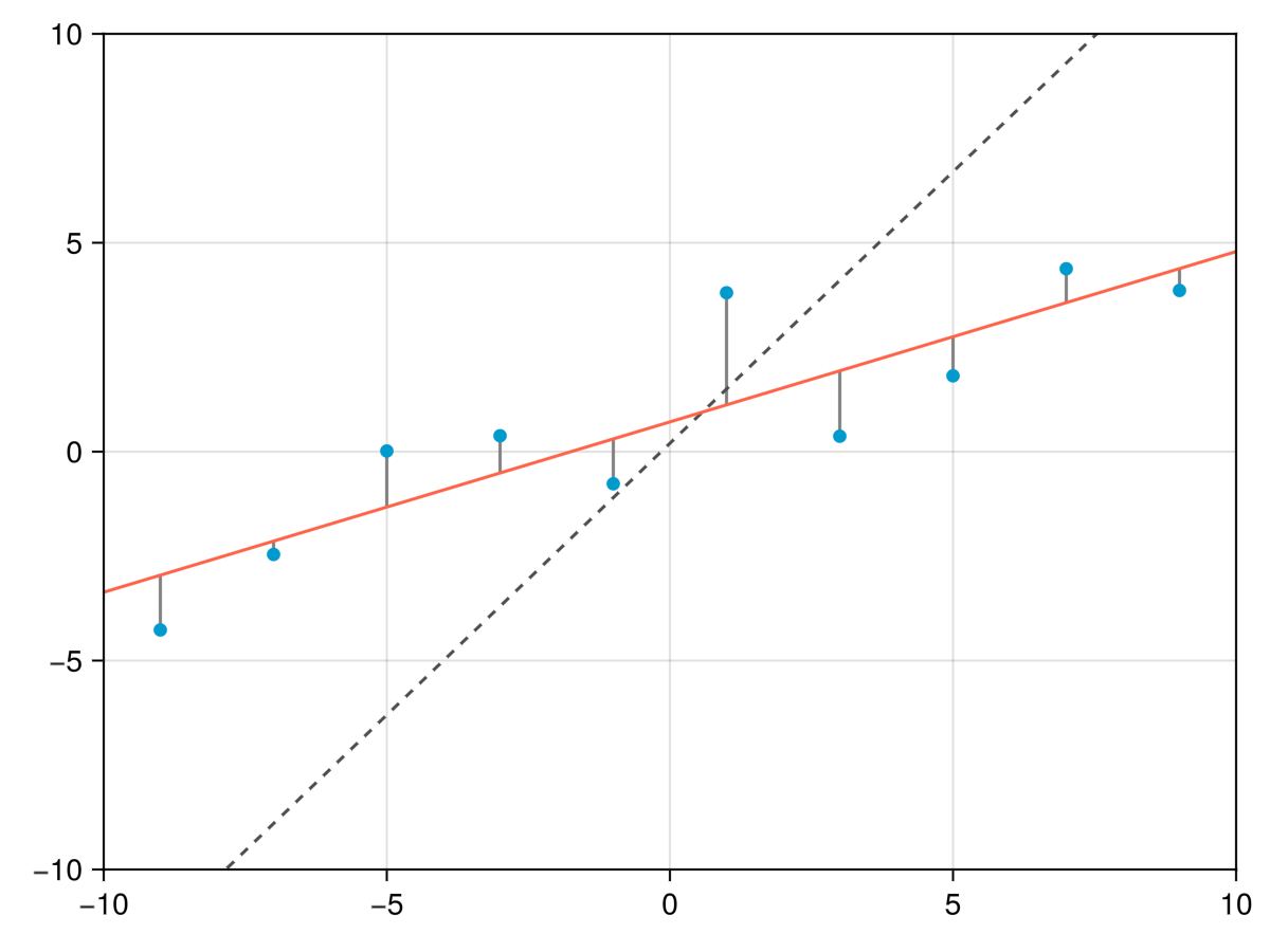
The example below shows a linear fit to randomly generated data, together with the residuals shown as lines between the data points and the fitted line. The line representing the initial guess parameters is shown as a dashed line.

Example: Lorentzian peak

Let’s say you take a noisy spectrum of a sample and observe a single peak around 500 nm. You have good reason to believe that the peak is Lorentzian in shape, a common line shape in spectroscopy. A Lorentzian line shape is given by the equation

$$L(x) = \frac{I_0}{1 + \left(\frac{x - x_0}{\Gamma / 2}\right)^2}$$

where $I_0$ is the amplitude, $x_0$ is the center frequency (often expressed in wavenumbers) of the peak, and $\Gamma$ is the full width at half maximum (FWHM) occurring at points $x = x_0 \pm \frac{\Gamma}{2}$.

Use CurveFit.jl’s NonlinearCurveFitProblem and solve to fit a Lorentzian function with the following parameters. The model function has the signature f(p, x) — parameter vector first, then the independent variable. After solving, retrieve the best-fit parameters with coef(sol) and their standard errors with stderror(sol).

A = 1.0
Γ = 28
x0 = 510

You should end up with something like below, depending on how many data points you create and how much noise you add to the data. Remember to include an error estimate for each parameter.

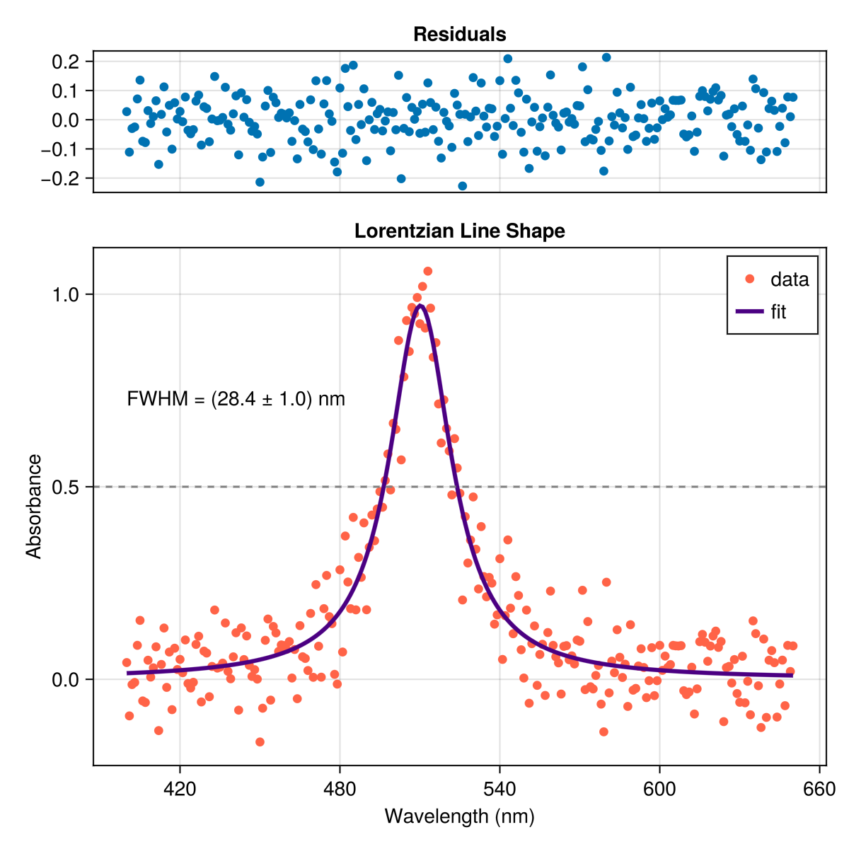
It is useful to plot the residuals of the fit to see how well the results fit the data. There should not be any systematic structure in the residuals. If there is, then the model is not a good fit to the data.

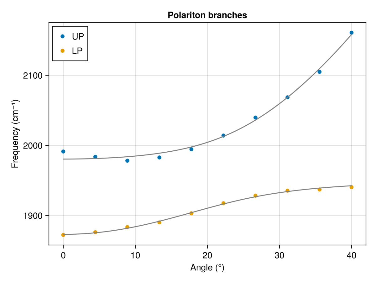
Example: polariton dispersion

Suppose you measure the Rabi splitting of a polariton system as a function of beam incidence angle. There will be two peaks in the transmission spectrum, one corresponding to the upper polariton and the other to the lower polariton, that will change in frequency with angle. One way to extract the Rabi splitting is to measure the angle-resolved spectrum, plot the frequency versus incidence angle, and fit the data to a simple coupled harmonic oscillator model, given by the Hamiltonian:

$$H_\text{total} = \begin{pmatrix} \omega_c(\theta) & 0 \\ 0 & \omega_v \end{pmatrix} + \begin{pmatrix} 0 & \Omega_R / 2 \\ \Omega_R / 2 & 0 \end{pmatrix} = \begin{pmatrix} \omega_c(\theta) & \Omega_R / 2 \\ \Omega_R / 2 & \omega_v \end{pmatrix}$$

Diagonalizing the Hamiltonian gives the upper and lower polariton energies:

$$\omega_\pm(\theta) = \frac{1}{2}\left[ \omega_c(\theta) + \omega_v \pm \sqrt{\left(\omega_c(\theta) - \omega_v\right)^2 + \Omega_R^2}\right]$$

The molecular vibrational transition is $\omega_v$, and the Rabi splitting magnitude is $\Omega_R$. The cavity mode frequency $\omega_c$ is given by the equation

$$\omega_c(\theta) = \omega_c(0)\left(1 - \frac{\sin^2\theta}{n^2} \right)^{-1/2}$$

where $\theta$ is the beam angle with respect to the normal of the cavity surface and $n$ is the refractive index of the intracavity medium.

Fitting the two polariton branches simultaneously just means writing one model function that returns both — we concatenate the upper and lower branch predictions with vcat and compare against the concatenated data.

using CurveFit

function cavity_mode_energy(θs, E_0, n)
    # Your code here
end

function polariton_branch(θs, E_v, E_0, n, Ω, branch)
    # Your code here — branch = +1 for UP, -1 for LP
end

function model(p, θs)
    E_v, E_0, n, Ω = p
    LP = polariton_branch(θs, E_v, E_0, n, Ω, -1)
    UP = polariton_branch(θs, E_v, E_0, n, Ω, +1)
    return vcat(LP, UP)
end

Then build a NonlinearCurveFitProblem and call solve().

prob = NonlinearCurveFitProblem(model, [E_v, E_0, n, Ω], θs, vcat(LP, UP))
sol = solve(prob)

The best-fit parameters are retrieved with coef(sol), and their standard errors with stderror(sol).

Problems

1. Fit the noisy Lorentzian spectrum described above. Report the peak position, FWHM, and amplitude with their standard errors.

2. Write the cavity_mode_energy and polariton_branch functions. Use them to generate data for the two polariton branches with Gaussian noise and parameters $\omega_c(0)$ = 1900 cm^-1, $\omega_v$ = 1950 cm^-1, $\Omega_R$ = 60 cm^-1, and $n$ = 1.4.

3. Build a NonlinearCurveFitProblem and call solve() to fit the model to the data. Try different initial guesses for the parameters and see how they affect the fit.

4. Try changing the number of fitting parameters. In the example above, we allowed four parameters to vary, but you can also fix some of them to known values. Often the molecular vibrational mode is known, for example. Remember to report the standard error on each parameter and the confidence intervals. What do these quantities mean?

Resources

• Least Squares Fitting on Wikipedia
• Khan Academy on residuals and least squares regression
• Ledvij, M. “Curve Fitting Made Easy.” Industrial Physicist 9, 24-27, Apr./May 2003.